7.4 Model binning

7.4.1 Model energy grid

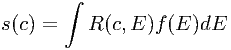
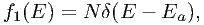
The spectrum of any X-ray source is given by its photon spectrum f(E). f(E) is a function of the continuous variable E, the photon energy, and has e.g. units of photons m^-2 s^-1 keV^-1. When we reconstruct how this source spectrum f(E) is observed by an instrument, f(E) is convolved with the instrument response R(c,E) in order to produce the observed count spectrum s(c) as follows:

(7.35)

where the variable c denotes the ”observed” (see below) photon energy and s has units of counts s^-1 keV^-1. The response function has the dimensions of an (effective) area, and can be given in e.g. m².

The variable c was denoted as the ”observed” photon energy, but in practice it is some electronic signal in the detector used, the strength of which usually cannot take arbitrary values, but can have only a limited set of discrete values. A good example of this is the pulse-height channel for a CCD detector.

In almost all circumstances it is not possible to do the integration in eqn. (7.35) analytically, due to the complexity of both the model spectrum and the instrument response. For that reason, the model spectrum is evaluated at a limited set of energies, corresponding to the same pre-defined set of energies that is used for the instrument response R(c,E). Then the integration in eqn. (7.35) is replaced by a summation. We call this limited set of energies the model energy grid or shortly the model grid. For each bin j of this model grid we define a lower and upper bin boundary E_1j and E_2j as well as a bin centroid E_j and a bin width ΔE_j, where of course E_j is the average of E_1j and E_2j, and ΔE_j = E_2j - E_1j.

Provided that the bin size of the model energy bins is sufficiently smaller than the spectral resolution of the instrument, the summation approximation to eqn. (7.35) is in general sufficiently accurate. The response function R(c,E) has therefore been replaced by a response matrix R_ij, where the first index i denotes the data channel, and the second index j the model energy bin number.

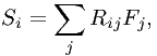
We have explicitly:

(7.36)

where now S_i is the observed count rate in counts/s for data channel i and F_j is the model spectrum (photons m^-2 s^-1) for model energy bin j.

This basic scheme is widely used and has been implemented e.g. in the XSPEC and SPEX (version 1.10 and below) packages.

7.4.2 Evaluation of the model spectrum

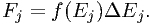
The model spectrum F_j can be evaluated in two ways. First, the model can be evaluated at the bin centroid E_j, taking essentially

(7.37)

This is appropriate for smooth continuum models like blackbody radiation, power laws etc. For line-like emission it is more appropriate to integrate the line flux within the bin analytically, and taking

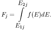(7.38)

Now a sometimes serious flaw occurs in most spectral analysis codes. The observed count spectrum S_i is evaluated straightforward using eqn. (7.36). Hereby it is assumed that all photons in the model bin j have exactly the energy E_j. This has to be done since all information on the energy distribution within the bin is lost and F_j is essentially only the total number of photons in the bin. Why is this a problem? It should not be a problem if the model bin width ΔE_j is sufficiently small. However, this is (most often) not the case.

Let us take an example. The standard response matrix for the ASCA SIS detector uses a uniform model grid with a bin size of 10 eV. At a photon energy of 1 keV, the spectral resolution (FWHM) of the instrument is about 50 eV, hence the line centroid of an isolated narrow line feature containing N counts can be determined with a statistical uncertainty of 50/2.35 eV (we assumed here for simplicity a Gaussian instrument response, for which the FWHM is approximately 2.35σ). Thus, for a moderately strong line of say 400 counts, the line centroid can be determined in principle with an accuracy of 1 eV, ten times better than the step size of the model energy grid. If the true line centroid is close to the boundary of the energy bin, there is a mis-match (shift) of 5 eV between the observed count spectrum and the predicted count spectrum, at about the 5σ significance level! If there are more of these lines in the spectrum, it is not excluded that never a satisfactory fit (in a χ² sense) is obtained, even in those cases where we know the true source spectrum and have a perfectly calibrated instrument! The problem becomes even more worrysome if e.g. detailed line-centroiding is done in order to derive velocity fields, like has been done e.g. for the Cas A supernova remnant.

A simple way to resolve these problems is just to increase the number of model bins. This robust method always works, but at the expense of a lot of computing time. For CCD-resolution spectra this is perhaps not a problem, but with the increased spectral resolution and sensitivity of the grating spectrometers of AXAF and XMM this becomes cumbersome.

For example, with a spectral resolution of 0.04 Å over the 5–38 Å band, the RGS detector of XMM will have a bandwidth of 825 resolution elements, which for a Gaussian response function translates into 1940 times σ. Several of the strongest sources to be observed by this instrument will have more than 10000 counts in the strongest spectral lines (example: Capella), and this makes it necessary to have a model energy grid bin size of about σ∕10000). The total number of model bins is then 194 000.

Most of the computing time in thermal plasma models stems from the evaluation of the continuum. The reason is that e.g. the recombination continuum has to be evaluated for all energies, for all relevant ions and for all relevant electronic subshells of each ion. On the other hand, the line power needs to be evaluated only once for each line, regardless of the number of energy bins. Therefore the computing time is approximately proportional to the number of bins. Going from ASCA-SIS resolution (1180 bins) to RGS resolution (194 000 bins) therefore implies more than a factor of 160 increase in computer time. And then it can be anticipated that due to the higher spectral resolution of the RGS more complex spectral models are needed in order to explain the observed spectra than are needed for ASCA, with more free parameters, which also leads to additional computing time. And finally, the response matrices of the RGS become extremely large. The RGS spectral response is approximately Gaussian in its core, but contains extended scattering wings due to the gratings, up to a distance of 0.5 Å from the line center. Therefore, for each energy the response matrix is significantly non-zero for at least some 100 data channels, giving rise to a response matrix of 20 million non-zero elements. In this way the convolution of the model spectrum with the instrument response becomes also a heavy burden.

For the AXAF-LETG grating the situation is even worse, given the wider energy range of that instrument as compared to the XMM-RGS.

Fortunately there are more sophisticated ways to evaluate the spectrum and convolve it with the instrument response, as is shown in the next subsection.

7.4.3 Binning the model spectrum

We have seen in the previous subsection that the ”classical” way to evaluate model spectra is to calculate the total number of photons in each model energy bin, and to act as if all flux is at the center of the bin. In practice, this implies that the ”true” spectrum f(E) within the bin is replaced by its zeroth order approximation f₀(E), given by

(7.39)

where N is the total number of photons in the bin, E_j the bin centroid as defined in the previous section and δ is the delta-function.

In this section we assume for simplicity that the instrument response is Gaussian, centered at the true photon energy and with a standard deviation σ. Many instruments have line spread functions with Gaussian cores. For instrument responses with extended wings (e.g. a Lorentz profile) the model binning is a less important problem, since in the wings all spectral details are washed out, and only the lsf core is important. For a Gaussian profile, the FWHM of the lsf is given by

(7.40)

How can we measure the error introduced by using the approximation (7.39)? Here we will compare the cumulative probability distribution function (cdf) of the true bin spectrum, convolved with the instrumental lsf, with the cdf of the approximation (7.39) convolved with the instrumental lsf. The comparison is done using a Kolmogorov-Smirnov test, which is amongst the most powerful tests in detecting the difference between probability distributions, and which we used successfully in the section on data binning. We denote the lsf-convolved cdf of the true spectrum by ϕ(c) and that of f₀ by ϕ₀(c). By definition, ϕ(-∞) = 0 and ϕ(∞) = 1, and similar for ϕ₀.

Similar to section 7.3, we denote the maximum absolute difference between ϕ and ϕ₀ by δ. Again, λ_k ≡δ should be kept sufficently small as compared to the expected statistical fluctuations D, where D is given again by eqn. (7.21). Following section 7.3 further, we divide the entire energy range into R resolution elements, in each of which a KS test is performed. For each of the resolution elements, we determine the maximum value for λ_k from (7.26)–(7.28), and using (7.34) we find for a given number of photons N_r in the resolution element the maximum allowed value for δ in the same resolution element.

The approximation f₀ to the true distribution f as given by eqn. (7.39) fails most seriously in the case that the true spectrum within the bin is also a δ-function, but located at the bin boundary, at a distance ΔE∕2 from the assumed line center at the bin center.

Using the Gaussian lsf, it is easy to show that the maximum error δ₀ for f₀ to be used in the Kolmogorov-Smirnov test is given by

(7.41)

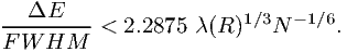
This approximation holds in the limit of ΔE ≪ σ. Inserting eqn. (7.40) we find that the bin size should be smaller than

(7.42)

Figure 7.6: Maximum model energy grid bin width ΔE in terms of the FWHM as a function of the number of photons N_r in the bin, using different approximations f₀ (solid line), f₁ (dashed line) and f₂ (dotted line) as discussed in the text. The calculation is done for R = 1 (upper curves) or R = 1000 (lower curves) resolution elements.

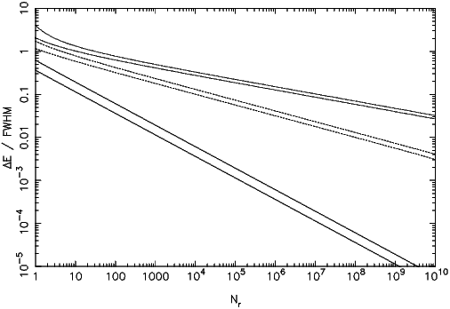
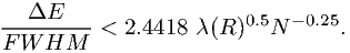
Exact numerical results are shown in fig. 7.6. The approximation (7.41) is a lower limit to the exact results, so can be safely used. A somewhat better approximation (but still a lower limit) appears to be the following:

(7.43)

As expected, one sees that for N = 10000 one needs to bin the model spectrum by about 0.01 times the FWHM.

A further refinement can be reached as follows. Instead of putting all photons at the bin center, we can put them at their average energy. This first-order approximation can be written as

(7.44)

where E_a is given by

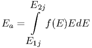(7.45)

In the worst case for approximation f₀ (namely a narrow line at the bin boundary) the approximation f₁ yields exact results. In fact, it is easy to see that the worst case for f₁ is a situation with two δ-lines of equal strength, one at each bin boundary. In that case the width of the resulting count spectrum ϕ₁ will be broader than σ. Again in the limit of small ΔE, it is easy to show that the maximum error δ₁ for f₁ to be used in the Kolmogorov-Smirnov test is given by

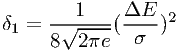(7.46)

where e is the base of the natural logarithms. Accordingly, the limiting bin size for f₁ is given by

(7.47)

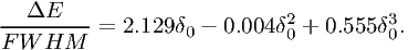
Exact results are plotted again in fig. 7.6. The better numerical approximation is

(7.48)

It is seen immediately that for large N the approximation f₁ requires a significantly smaller number of bins than f₀.

We can improve further by not only calculating the average energy of the photons in the bin (the first moment of the photon distribution), but also its variance (the second moment).

In this case we approximate

(7.49)

where τ is given by

(7.50)

The resulting count spectrum is then simply Gaussian, with the average value centered at E_a and the width slightly larger than the instrumental width σ, namely .

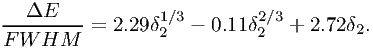
The worst case for f₀ again occurs for two δ-lines at the opposite bin boundaries, but now with unequal strength. It can be shown again in the small bin width limit that

(7.51)

and that this maximum occurs for a line ratio of 6 - 1. The limiting bin size for f₂ is given by

(7.52)

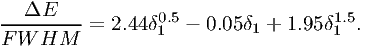
Exact results are plotted again in fig. 7.6. The better numerical approximation is

(7.53)

7.4.4 Which approximation to choose?

It is now time to compare the different approximations f₀, f₁ and f₂ as derived in the previous subsection. It can be seen from fig. 7.6 that the approximation f₁ implies an order of magnitude or more improvement over the classical approximation f₀. However, the approximation f₂ is only slightly better than f₁. Moreover, the computational burden of approximation f₂ is large. The evaluation of (7.50) is rather straightforward to do, although care should be taken with single machine precision: first the average energy E_a should be determined, and then this value should be used in the estimation of τ. A more serious problem is that the width of the lsf should be adjusted from σ to . If the lsf is a pure Gaussian, this can be done analytically; however for a slightly non-Gaussian lsf the true lsf should be convolved in general numerically with a Gaussian of width τ in order to obtain the effective lsf for the particular bin, and the computational burden is quite heavy. On the other hand, for f₁ only a shift in the lsf is sufficient.

Therefore we recommend here to use the linear approximation f₁. The optimum bin size is thus given by (7.28), (7.34) and (7.48).

7.4.5 The effective area

In the previous subsection we have seen how the optimum model energy grid can be determined, taking into account the possible presence of narrow spectral features, the number of resolution elements and the flux of the source. There remains one other factor to be taken into account, and that is the energy dependence of the effective area. In the previous section we have considered merely the effect of the spectral redistribution (”rmf” in XSPEC terms), here we consider the ”arf”.

If the effective area A_j(E) would be a constant A_j for a given model bin j, and if the photon flux of the bin in photons m^-2 s^-1 would be given by F_j, then the total count rate produced by this bin would be simply A_jF_j. This approach is actually used in the ”classical” way of analysing spectra, and it is justified in the approximation that all photons of the model bin would have the energy of the bin centroid. This is not always the case, however, and in the previous subsection we have given arguments that it is better not only to take into account the flux F_j but also the average energy E_a of the photons within the model bin. This average energy E_a is in general not equal to the bin centroid E_j, and hence we need to evaluate the effective area not at E_j but at E_a.

In general the effective area is energy-dependent and it is not trivial that the constant approximation over the width of a model bin is justified. In several cases this will not be the case. We consider here the most natural first-order extension, namely the assumption that the effective area within a model bin is a linear function of the energy. For each model bin j, we write the effective area A(E) in general as follows:

(7.54)

The above approximation is good when the residuals ϵ_j(E) are sufficiently small. We use a Taylor expansion in order to estimate the residuals:

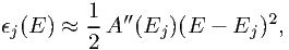(7.55)

where as usual A^′′ denotes the second derivative of A with respect to the energy. It is immediately seen from the above expressions that the maximum error occurs when E is at one of the bin boundaries. As a consequence, we can estimate the maximum error ϵ_max as:

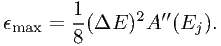(7.56)

By using the approximation (7.54) with ϵ neglected we therefore make at most a maximum error given by (7.56) in the effective area. This can be translated directly into an error in the predicted count rate by multiplying ϵ_max by the photon flux F_j. Alternatively, dividing ϵ_max by the effective area A_0j at the bin center, we get the maximum error in the predicted probability distribution for the resulting counts. This maximum can be taken also as the maximum deviation δ in the cumulative distribution function that we used in the previous sections in the framework of the Kolmogorov-Smirnov tests.

Hence we write

(7.57)

Using the same theory as in the previous section, we find an expression for the optimum bin size, as far as the effective area is treated in the linear approximation (compare with eqn. (7.47)):

(7.58)

The bin width constraint derived here depends upon the dimensionless curvature of the effective area A∕E_j²A^′′. In most parts of the energy range this will be a number of order unity or less. Since the second prefactor E_j∕FWHM is by definition the resolution of the instrument, we see by comparing (7.58) with (7.47) that in general (7.47) gives the most severe constraint upon the bin width, unless either the resolution gets small (what happens e.g. for the Rosat PSPC detector at low energies), or the effective area curvature gets large (what may happen e.g. near the exponential cut-offs caused by filters).

Large effective area curvature due to the presence of exponential cut-offs is usually not a very serious problem, since these cut-offs also cause the count rate to be very low and hence weaken the binning requirements. Of course, discrete edges in the effective area should always be avoided in the sence that edges should always coincide with bin boundaries.

In practice, it is a little complicated to estimate from e.g. a look-up table of the effective area its curvature, although this is not impossible. As a simplification for order of magnitude estimates we can use the case where A(E) = A₀e^bE locally, which after differentiation yields

(7.59)

Inserting this into (7.58), we obtain

(7.60)

7.4.6 Final remarks

In the previous two subsections we have given the constraints for determining the optimal model energy grid. Combining both requirements (7.48) and (7.60) we obtain the following optimum bin size:

(7.61)

where w₁ and w_a are the values of ΔE/FWHM as calculated using (7.48) and (7.60), respectively.

This choice of model binning ensures that no significant errors are made either due to inaccuracies in the model or effective area for flux distributions within the model bins that have E_a≠E_j.